Chutes and Ladders (or Snakes and Ladders in some parts?) is a children’s board game where the goal is to make your way through 100 squares/spaces to the end of the board first. If you’re not familiar, look up an image of the game board to get an idea.
As a player, the strategy is to … oh wait, you just spin the wheel, don’t think at all, and move squares. More specifically you spin an integer between 1 and 6, move that many squares, follow chutes or ladders, and repeat until finished. There is literally no strategy or decision making in the entire game.
This makes the game pretty strategically boring, but also very amenable to statistical analysis. And honestly, my main gripe with the game isn’t the boredom, it’s that it seems to have the potential to take way more turns than is appropriate for a game that claims to be for 3-year-olds.
And so, let’s model Chutes and Ladders!
First things first, we can construct a transition matrix that describes the probability of landing on any square given a starting square. The spinner has equal chance of getting the integers 1 – 6. If you land on a normal square, you stay there and if you land on the start of 1 of the 10 chutes (which move backward on the board) or 1 of the 9 ladders (which move forward on the board) we’ll say you instead wind up on the end of the chute/ladder. You always leave the first square (number 0) and can never return to it. Conversely, if you land on the last square (number 100), you’ll never leave.
So we can construct a \( 101 \times 101 \) matrix where each entry \( T_{ij} \) is the probability of starting on square \( i \) and ending on square \( j \).
Using this transition matrix, one nice thing to compute is the probability of being on the different squares at each turn (for just 1 player). We can start with a probability vector that had probability 1 on the start square and “taking a turn” corresponds to multiplying the vector by the transition matrix
\( p_{t+1} = p_t \cdot T \).
We can iterate many times and see what the distribution looks like.
I made the probability of being on square 100 (done with the game) in red on the right. As a parent, it concerns me how slowly this bar rises after about turn 10 … just hanging out below 0.2. This is a game for 3 year olds!
Another view of this is to ask: how long does it take to win the game? What does this distribution of game times look like? We can also use the transition matrix to simulate games, not just update probability distributions. If we simulate 10,00 chutes and ladders players, we can plot how many games take \( N \) turns or more. We can also track \( 1 – p(100) \) from the animation (1 minus the red bar value) and these should agree.
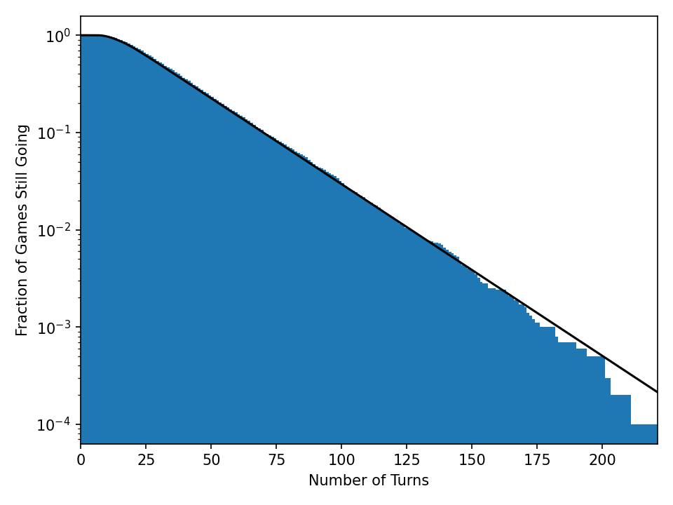
Something like 10% of games take 75 turns. Oof. It’s worse when 4 players are playing and you think about how long it takes the last player to finish.
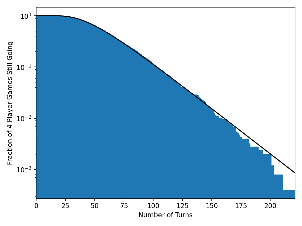
Simulation (blue histogram) and exact computation (black line) of game length distribution for 4 players.
Now 10% of games take 100 turns for all players to finish. Maybe it’s just me, but I feel like if you’re designing games for 3-year-olds, you have some responsibility to run a handful of Monte-Carlo simulations to get a sense of how laborious getting through an entire play-through will be.