Chutes and Ladders (or Snakes and Ladders in some parts?) is a children’s board game where the goal is to make your way through 100 squares/spaces to the end of the board first. If you’re not familiar, look up an image of the game board to get an idea.
As a player, the strategy is to … oh wait, you just spin the wheel, don’t think at all, and move squares. More specifically you spin an integer between 1 and 6, move that many squares, follow chutes or ladders, and repeat until finished. There is literally no strategy or decision making in the entire game.
This makes the game pretty strategically boring, but also very amenable to statistical analysis. And honestly, my main gripe with the game isn’t the boredom, it’s that it seems to have the potential to take way more turns than is appropriate for a game that claims to be for 3-year-olds.
And so, let’s model Chutes and Ladders!
First things first, we can construct a transition matrix that describes the probability of landing on any square given a starting square. The spinner has equal chance of getting the integers 1 – 6. If you land on a normal square, you stay there and if you land on the start of 1 of the 10 chutes (which move backward on the board) or 1 of the 9 ladders (which move forward on the board) we’ll say you instead wind up on the end of the chute/ladder. You always leave the first square (number 0) and can never return to it. Conversely, if you land on the last square (number 100), you’ll never leave.
So we can construct a \( 101 \times 101 \) matrix where each entry \( T_{ij} \) is the probability of starting on square \( i \) and ending on square \( j \).
Image showing the Chutes and Ladders transition matrix. White is probability-zero and black is probability-one. Looking at a row tells you the squared you might land on starting from the square that has that row’s index.
Using this transition matrix, one nice thing to compute is the probability of being on the different squares at each turn (for just 1 player). We can start with a probability vector that had probability 1 on the start square and “taking a turn” corresponds to multiplying the vector by the transition matrix
\( p_{t+1} = p_t \cdot T \).
We can iterate many times and see what the distribution looks like.
GIF of the probability of being on each square as a function of the turn number. You may need to click on the image to make the animation go.
I made the probability of being on square 100 (done with the game) in red on the right. As a parent, it concerns me how slowly this bar rises after about turn 10 … just hanging out below 0.2. This is a game for 3 year olds!
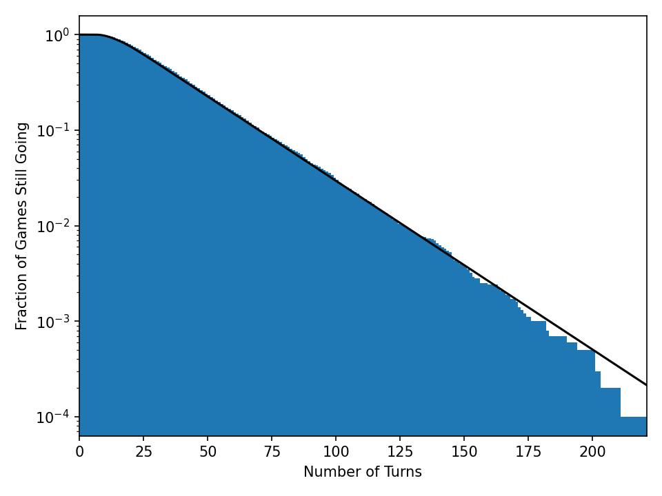
Another view of this is to ask: how long does it take to win the game? What does this distribution of game times look like? We can also use the transition matrix to simulate games, not just update probability distributions. If we simulate 10,00 chutes and ladders players, we can plot how many games take \( N \) turns or more. We can also track \( 1 – p(100) \) from the animation (1 minus the red bar value) and these should agree.
Simulation (blue histogram) and exact computation (black line) of game length distribution for single players.
Something like 10% of games take 75 turns. Oof. It’s worse when 4 players are playing and you think about how long it takes the last player to finish.
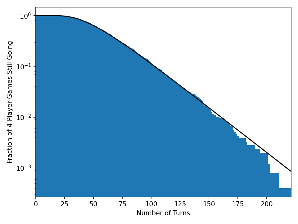
Simulation (blue histogram) and exact computation (black line) of game length distribution for 4 players.
Now 10% of games take 100 turns for all players to finish. Maybe it’s just me, but I feel like if you’re designing games for 3-year-olds, you have some responsibility to run a handful of Monte-Carlo simulations to get a sense of how laborious getting through an entire play-through will be.
At first glance, it looks like the demographics of the US Senate are not representative of the US as a whole; the demographic percentages are not very similar to the Senate percentages. But how can we check this quantitatively? The p-value, a simple metric coined by statisticians, is commonly used by researchers in science, economics, sociology, and other fields to test how consistent a measurement or finding is with a model of the world they are considering.
It’s important to note that this is an overly simplistic picture of demographics. This categorization of gender and race leaves out many identities which are common. This simplified demographic information happens to be easy to come by, but this analysis could easily be extended to include more nuanced data on gender and race, disability identity or sexual orientation, or other factors like socio-economic background, geography, etc. if it is available for the Senate and the state populations.
First, a bit of statistics and probability background.
Randomness and biased coin flips
In many domains (physics, economics, sociology, etc.) it is assumed that many measurements or findings have an element of randomness or unpredictability. This randomness can be thought of as intrinsic to the system, as is often the case in quantum mechanics, or as the result of missing measurements, e.g. what I choose to eat for breakfast on Tuesday might be more predictable if you know what I ate for breakfast on Monday. Another simple example is a coin flip: if the coin is “fair” you know that you’ll get heads and tails half of the time each, but for a specific coin flip, there is no way of knowing whether you’ll get heads or tails. It turns out that sub-atomic particle interactions, what you buy at the supermarket on a given day, or who becomes part of your social circle all have degrees of randomness. Because of this randomness, it becomes hard to make exact statements about systems that you might study.
For example, let’s say you find a quarter and want to determine whether the coin was fair, i.e. it would give heads and tails half of the time each. If you flip the coin 10 times, you might get 5 heads and 5 tails, which seems pretty even. But you might also get 7 heads and 3 tails. Would you assume that this coin is biased based on this measurement? Probably not. One way of thinking about this would be to phrase the question as: what are the odds that a fair coin would give me this result? It turns out that with a fair coin, the odds of getting 5 heads is about 25% and the odds of getting 7 heads is about 12%. Both of these outcomes are pretty likely with a fair coin and so neither of them really lead us to believe that the coin is not fair. Try flipping a coin 10 times; how many heads do you get?
Let’s say you now flip the coin 100 times. The odds of getting 50 heads is about 8%. But the odds of getting 70 heads is about .002%! So if you rolled 70 heads, you would only expect that to happen 2 out of every 100,000. That’s pretty unlikely and would probably lead you to believe that the coin is actually biased towards heads.
This quantity: the odds that a model (a fair coin in this example) would produce a measurement or finding (70 heads in this example) is often called a p-value. We can use this quantity to estimate how likely it is that the current US Senate was generated by a “fair” process. In order to do that, we’ll first need to define what it means (in a probabilistic sense) for the process of selecting the US Senate to be “fair”. Similarly, we had to define that a “fair” coin was one that gave us equal odds of heads and tails for each toss. Now you can start to apply this tool to the Senate data.
What is “fairness” in the US Senate
I’m going to switch into the first person for a moment since the choices in this paragraph are somewhat subjective. I have a particular set of principles that are going to guide my definition of “fair”. You could define it in some other way, but it would need to lead to a quantitative, probabilistic model of the Senate selection process in order to assess how likely the current Senate is. The way I’m going to define “fair” representation in the US Senate comes from the following line of reasoning. I believe that, in general, people are best equipped to represent themselves. I also believe that senators should be representing their constituents, i.e. the populations of their states. Taking these two things together, this means that I think that the US Senate should be demographically representative on a per-state basis. I don’t mean this strictly such that since women are 51% of the population there should be exactly 51 women senators, but in a random sense such that if a state is 51% women, the odds of electing a woman senator should be 51%. See the end of this post for a few assumptions this model makes.
Given this definition of “fair”, we can now assess how likely or unlikely is it that a fair process would lead to the Senate described above: 1 Black woman senator, 3 Black senators, 21 women senators, or 3 states with 2 women senators. To do this we’ll need to get the demographic information, per state, for the fraction of the state that is women and Black. I’m getting this information from the 2010 Census. It is possible to calculate these probabilities exactly, but it becomes tricky because, for instance, there are many different ways that 21 women could be elected (there are about 2,000 billion-billion different ways), and so going through all of them is very difficult. Even if you could calculate 1 billion ways per second, it would still take you, 60,000 years to finish. If we just want a close approximation to the probability, we can use a trick called “bootstrapping” in statistics. This works by running many simulations of our fair model of the Senate and then checking to see how many of these simulations have outcomes like 21 women senators or 3 Black senators. Depending on how small the probabilities we are interested are, we can often get away with only running millions or billions of simulations, which seems like a lot but is much easier than having to do many billion-billion calculations and can usually be done in a matter of minutes or hours.
The core process of generating these simulations is equivalent to flipping a bunch of biased coins. For each state, we know the fraction of the population which are women and/or Black. So, for each of the two Senate seats per state, we flip two coins. One coin determines gender and the other race. We can then do this for all 50 states. Now we have one simulation and we can check how many Black women senators or states with 2 women senators, etc., we have. We can then repeat this process millions or billions of times so that we can estimate the full distribution of outcomes. Once we have this estimated distribution, we can check to see how often we get outcomes as far away or further from the expected average.
So, what are the odds?
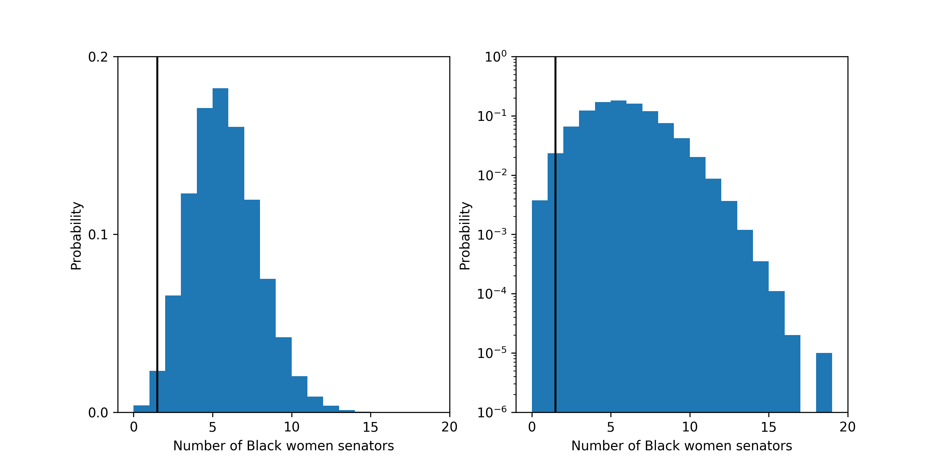
So what do the results look like? I’m going to present two plots side-by-side which show the same information in two ways. The plots on the left will show the distributions of expected outcomes the fair process predicts as blue histograms and where the current Senate value falls in that distributions as a black vertical line. The plots on the right will show the same information with the y-axis log-scaled. This will make it easier to see very small probabilities, but also visually warps the data to make small probabilities appear larger than that really are. If you’re not used to looking at log-scale plots, the plot on the left gives the clearest picture of the data. Data and code to reproduce these figures can be found here.
First, let’s look at what the probability is that a fair process produced a Senate with 1 or fewer Black women senators. The probability is about 2.7 in 100. The most likely outcome predicted by a fair process is 5 Black women senators which should happen 13% of the time.
The probability distribution for the number of Black Women senators under the fair model. Left plot is linear y-scale and right plots is log y-scale. The vertical black line shows the current number of Black women: 1, in the Senate.
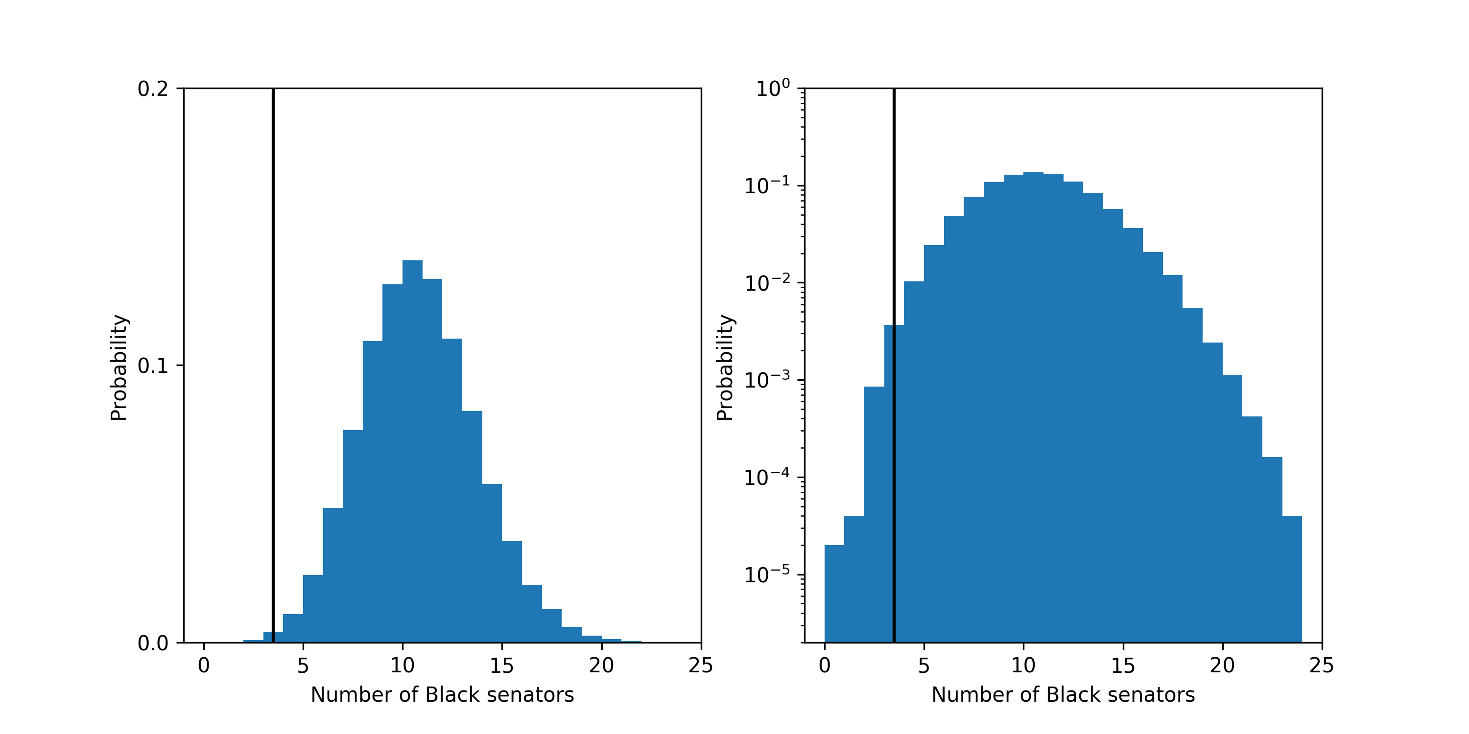
The probability that a fair process led to a Senate with 3 or fewer Black senators is about 4.6 in 1,000. The most likely outcome predicted by a fair process is 10 Black senators which should happen about 14% of the time.
The probability distribution for the number of Black senators under the fair model. Left plot is linear y-scale and right plots is log y-scale. The vertical black line shows the current number of Black people: 3, in the Senate.
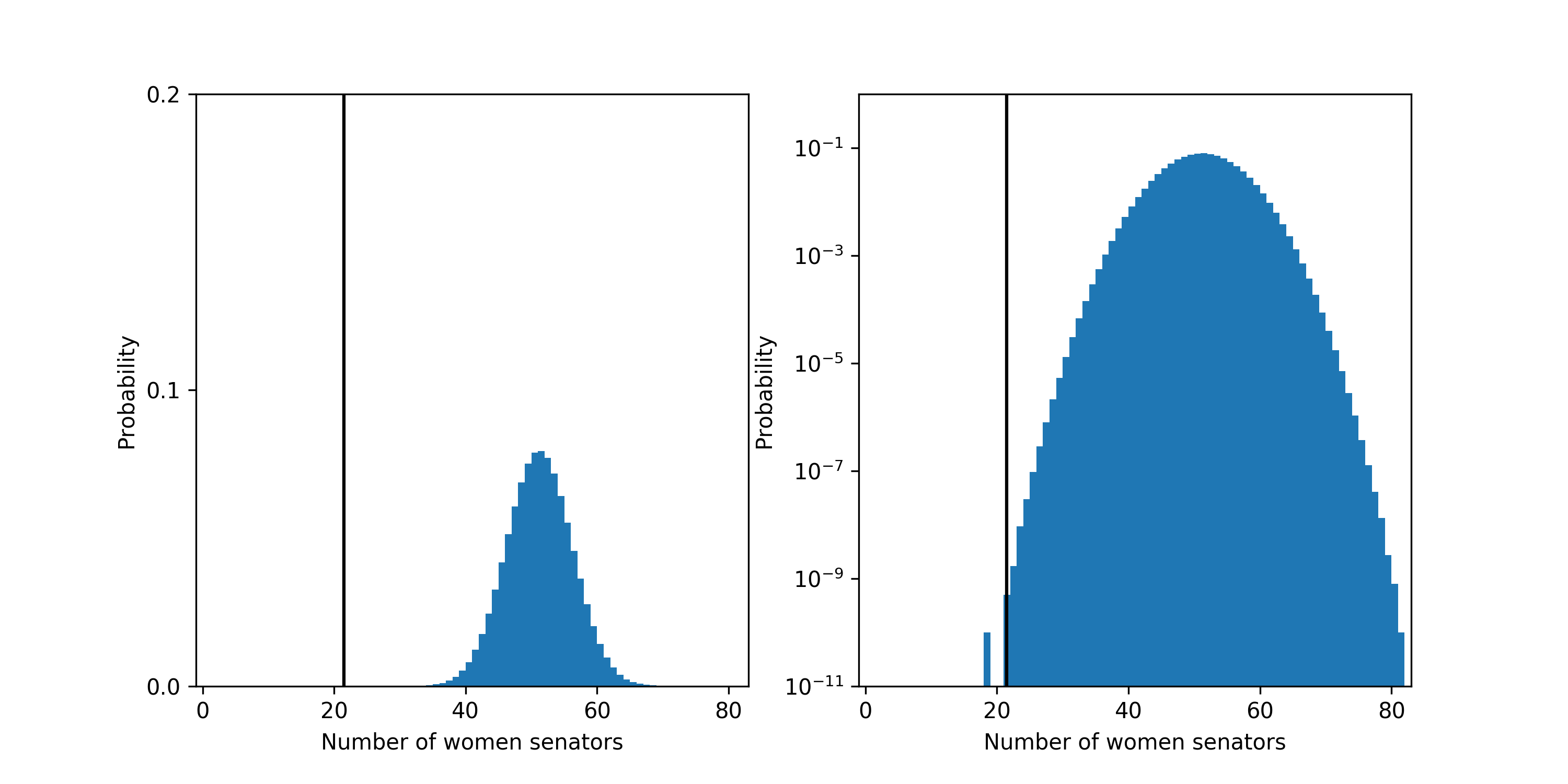
The probability that a fair process led to a Senate with 21 or fewer women senators is about 6 in 10,000,000,000! The most likely outcome predicted by a fair process is 51 women senators which should happen about 8% of the time.
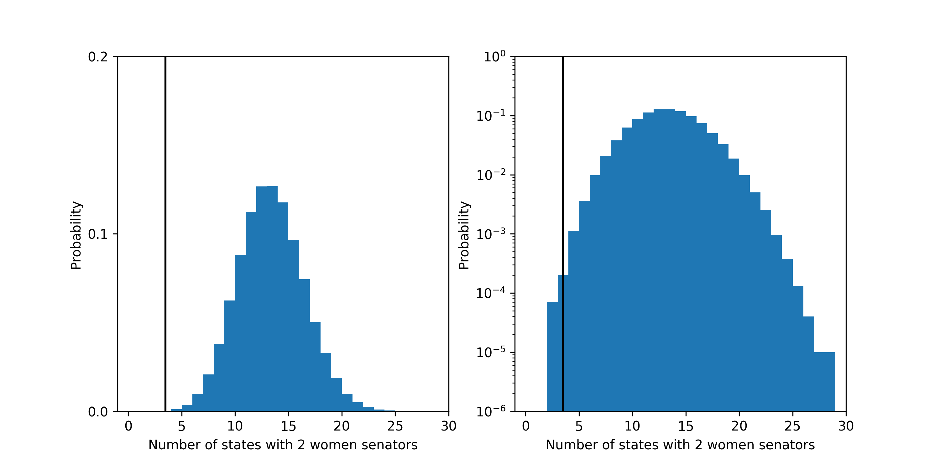
Finally, the probability that a fair process led to a Senate with 3 or fewer states with 2 women senators is about 3 in 10,000. The most likely outcome predicted by a fair process is 13 state with 2 women senators which should happen about 13% of the time.
The probability distribution for the number of states with 2 women senators under the fair model. Left plot is linear y-scale and right plots is log y-scale. The vertical black line shows the current number of states: 3, in the Senate.
These odds together show that it is very unlikely that the process for selecting US senators is fair according the the definition I have chosen. Now the question becomes: how does this disparity arise?
There is a wealth of evidence that shows how this comes about, such as segregation in schools and housing, unequal access to employment and social networks, gerrymandering, racial discrimination in voting through voter ID laws, and the repeal of portions of the voting rights act, just to name a few.
Nate Silver did a bit of analysis to trying to understand this (thanks for the reference, Peter). In 2009, he wrote a post titled: Why Are There No Black Senators? The main finding is that there is a nonlinear relationship between district demographics and House representative demographics. If a district is less than about 35% Black, the district has a lower probability of electing a Black rep. than would be expected by demographics. Conversely, if a district is more than about 35% Black, it is slightly more likely to elect a Black representative than would be expected by demographics. Unfortunately, I think he does a fairly bad job at trying to explain the finding, but the finding itself is interesting.
Silver then asks whether these racial biases in House voting patterns can explain the lack of Black senators.
They essentially do. Since states are more homogeneous than House districts, the fraction of state populations that are Black are much smaller than 35%. In fact, only one state has more than a 35% Black population (Mississippi at 37%). This means that Silver’s model predicts that there should only be about 1 Black senator, which is consistent with the 0 Black senators at the time and the 3 Black senators now. That data wasn’t published with the article, so it’s hard to say what the exact odds of 0 or 3 would be, but approximating it as a Poisson distribution gives 30% and 10% respectively.
Another way of trying to get at this question is to split the process of becoming a senator into two parts and look for bias in the parts individually. The first is the path that leads people to becoming candidates for Senate seats and the second is the election process which choses senators from this pool. This data is not easily available on the internet as far as I can tell (Let me know if that’s not true!), but would shed more light on where the biases are coming in to the process.
Assumptions and comments
A few assumptions that I am making:
the 2010 demographics are similar to the demographics of today,
the product of the gender and race fractions give the gender-race fractions per state,
the census demographics are similar to the demographics of those eligible to be a senator per state, and
that all senators are elected at once.
I’ve compared assuming flat demographics across states and the data that I use above and the p-values fluctuated up or down about a factor of 2 or 3. If I could get data that doesn’t make the above assumptions, I wouldn’t expect anything to change by more than another factor of 2 or 3 up or down.
Edit: The 6 in 10,000,000,000 statistic is probably not super accurate since it happens so rarely (it’s way out in the tail of the distribution). I’m confident that it is smaller than 1 in 100,000,000 but wouldn’t claim the number I’m reporting is super accurate.
And a comment:
The statement “I believe that, in general, people are best equipped to represent themselves” needs a bit of unpacking. I would probably add the condition that, given equal access to resources, people are generally best equipped to represent themselves. I also think the idea that “some people are intrinsically more likely to want to be a senator” is kind of the reverse of the way I’m looking at the problem. Representatives and senators should represent their constituents. Given that I also think that people are best equipped to represent themselves, the jobs of Congress should be adapted so that more people could fulfill them. Congress already receives a ton of support from staff and experts, so it is not clear to me that it requires a particular set of skills or level of expertise apart from the intention to represent your constituents.
Thanks to Sarah for edits and feedback! Thanks Mara, Papa, and Dimitri for catching some typos!
Machine learning is a broad set of techniques which can be used to identify patterns in data and use these patterns to help with some task like early seizure-detection/prediction, automated image captioning, automatic translation, etc. Most machine learning techniques have a set of parameters which need to be tuned. Many of these techniques rely on a very simple idea from calculus in order to tune these parameters.
Machine learning is a mapping problem
Machine learning algorithms generally have a set of parameters, which we’ll call \(\theta\), that need to be tuned in order for the algorithm to perform well at a particular task. An important question in machine learning is how to choose the parameters, \(\theta\), so that my algorithm performs the task well. Let’s look at a broad class of machine learning algorithms which take in some data, \(X\), and use that data to make a prediction, \(\hat y\). The algorithm can be represented by a function which makes these predictions,
\( \hat y = f(X;\theta)\).
This notation means that we have some function or mapping \(f(.; \theta)\) which has parameters \(\theta\). Given some piece of data \(X\), the algorithm will made some prediction \(\hat y\). If we change the parameters, \(\theta\), then the function will produce a different prediction.
If we choose random values for \(\theta\), there is no reason to believe that our mapping, \(f(.; \theta)\), will do anything useful. But, in machine learning, we always have some training data which we can use to tune the parameters, \(\theta\). This training data will have a bunch of input data which we can label as: \(X_i,\ i \in 1,\ 2,\ 3,\ldots\), and a bunch of paired labels: \(y_i,\ i \in 1,\ 2,\ 3,\ldots\), where \(y_i\) is the correct prediction for \(X_i\). Often, this training data has either been created by a simulation or labeled by hand (which is generally very time/money consuming).
Learning is parameter tuning
Now that we have ground-truth labels, \(y_i\), for our training data, \(X_i\), we can then evaluate how bad our mapping, \(f(.; \theta)\), is. There are many possible ways to measure how bad \(f(.; \theta)\) is, but a simple one is to compare the prediction of the mapping \(\hat y_i\) to the ground-truth label \(y_i\),
\( y_i-\hat y_i \).
Generally, mistakes which cause this error to be positive or negative are equally bad so a good measure of the error would be:
\(( y_i-\hat y_i)^2 =( y_i-f(X_i;\theta))^2\).
When this quantity is equal to zero for every piece of data we are doing a perfect mapping, and the larger this quantity is the worse our function is at prediction. Let’s call this quantity summed over all of the training data the error
\(E(\theta)=\sum_i( y_i-f(X_i;\theta))^2\).
So, how do we make this quantity small? One simple idea from calculus is called gradient descent. If we can calculate the derivative or gradient of the error with respect to \(\theta\) then we know that if we go in the opposite direction (downhill), then our error should be smaller. In order to calculate this derivative, our mapping, \(f(.,\theta)\), needs to be differentiable with respect to \(\theta\).
So, if we have a differentiable \(f(.,\theta)\) we can compute the gradient of the cost function with respect to \(\theta\)
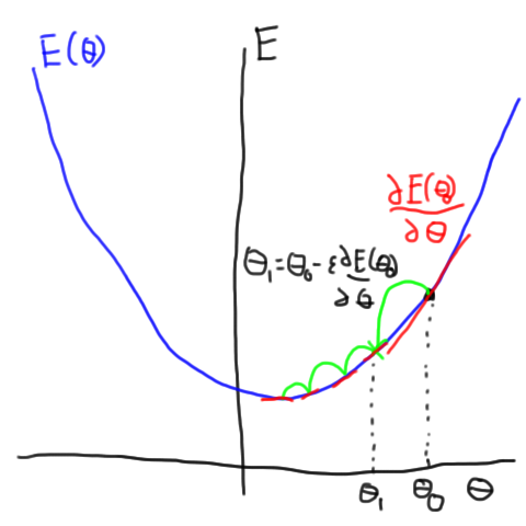
where \(\epsilon\) is a small scalar. Now, if we repeat this process over and over, the value of the error, \(E(\theta)\) should get smaller and smaller as we keep updating \(\theta\). Eventually, we should get to a (local) minimum at which point our gradients will become zero and we can stop updating the parameters. This process is shown (in a somewhat cartoon way) in this figure.
If the error function is shaped somewhat like a bowl as a function of some parameter theta, we can calculate the derivative of the bowl and walk downhill to the bottom.
Extensions and exceptions
This post presented a slightly simplified picture of learning in machine learning. I’ll briefly mention a few of the simplifications.
The terms error function, objective function, and cost function are all used basically interchangeably in machine learning. In probabilistic models you may also see likelihoods or log-likelihoods which are similar to a cost function except they are setup to be maximized rather than minimized. Since people (physicists?) like to minimize things, negative log-likelihoods are also used.
The squared-error function was a somewhat arbitrary choice of error function. It turns out that depending on what sort of problem you are working on, e.g. classification or regression, you may want a different type of cost function. Many of the commonly used error function can be derived from the idea of maximum likelihood learning in statistics.
There are many extensions to simple gradient descent which are more commonly used such as stochastic gradient descent (sgd), sgd with momentum and other fancier things like Adam, second-order methods, and many more methods.
Not all learning techniques for all models are (or were initially) done through gradient descent. The first learning rule for Hopfield networks was not based on gradient descent although the proof of the convergence of inference was based on (not-gradient) descent. Infact, it has been replaced with a more modern version based on gradient descent of an objective function.
In Part 2, we adapted three tools developed for vectors to functions: a Basis in which to represent our function, Projection Operators to find the components of our function, and a FunctionRebuilder which allows us to recreate our vector in the new basis. This is the third (and final!) post in a series of three:
We can apply these tools to two problems that are common in Fourier Series analysis. First we’ll look at the square wave and then the sawtooth wave. Since we’ve chosen a sine and cosine basis (a frequency basis), there are a few questions we can ask ourselves before we begin:
Will these two functions contain a finite or infinite number of components?
Will the amplitude of the components grow or shrink as a function of their frequency?
Let’s try and get an intuitive answer to these questions first.
For 1., another way of asking this question is “could you come up with a way to combine a few sines and cosines to create the function?” The smoking guns here are the corners. Sines and cosines do not have sharp corners and so making a square wave or sawtooth wave with a finite number of them should be impossible.
For 2., one way of thinking about this is that the function we are decomposing are mostly smooth with a few corners. To get them to be smooth, we can’t have more and more high frequency components, so the amplitude of the components should shrink.
Let’s see if these intuitive answers are borne out.
Square Wave
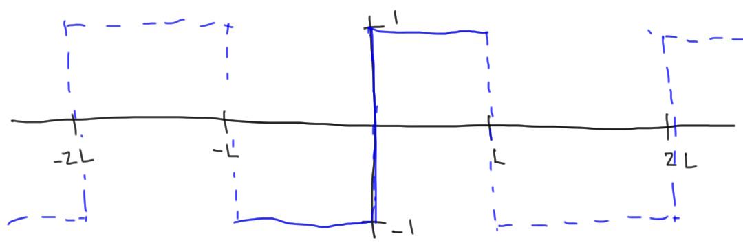
We’ll center the square wave vertically at zero and let it range from \([-L, L]\). In this case, the square wave function is
If we imagine this function being repeated periodically outside the range \([-L, L]\), it would be an odd (antisymmetric) function. Since sine functions are odd and cosine functions are even, an arbitrary odd function should only be built out of sums of other odd functions. So, we get to take one shortcut and only look at the projections onto the sine function (the cosine projections will be zero). You should work this out if this explanation wasn’t clear.
Since the square wave is defined piecewise, our projection integral will also be piecewise:
In Part 1, we developed three tools: a Basis in which to represent our vectors, Projection Operators to find the components of our vector, and a VectorRebuilder which allows us to recreate our vector in the new basis. This is the second post is a series of three:
We now want to develop these tools and apply the intuition to Fourier Series. The goal will be to represent a function (vectors) as the sum of sines and cosines (our basis). To do this we will need to define a basis, create projection operators, and create a functions rebuilder.
We will restrict ourselves to functions on the interval: \([-L,L]\). A more general technique is the Fourier Transform, which can be applied to functions on more general intervals. Many of the ideas we develop for Fourier Series can be applied to Fourier Transforms.
Note: I originally wrote this post with the interval \([0,L]\). It’s more standard (and a bit easier) to use \([-L,L]\), so I’ve since changed things to this convention. Video has not been updated, sorry :/
Choosing Basis Functions
Our first task will be to choose a set of basis function. We have some freedom to choose a basis as long as each basis function is normalized and is orthogonal to every other basis function (an orthonormal basis!). To check this, we need to define something equivalent to the dot product for vectors. A dot product tells us how much two vectors overlap. A similar operation for functions is integration.
Let’s look at the integral of two functions multiplied together over the interval: \([-L, L]\). This will be our guess for the definition of a dot product for functions, but it is just a guess.
\(\int_{-L}^Ldx~f(x)g(x)\)
If we imagine discretizing the integral, the integral becomes a sum of values from \(f(x)\) multiplied by values of \(g(x)\), which smells a lot like a dot product. In the companion video, I’ll look more at this intuition.
Now, we get to make another guess. We could choose many different basis functions in principle. Our motivation will be our knowledge that we already think about many things in terms of a frequency basis, e.g. sound, light, planetary motion. Based on this motivation, we’ll let our basis functions be:
\(s_n(x) = A_n \sin(\frac{n\pi x}{L})\)
and
\(c_n(x) = B_n \cos(\frac{n\pi x}{L})\).
We need to normalize these basis functions and check that they are orthogonal. Both of these can be done through some quick integrals using Wolfram Alpha. We get
This is a different convention from what is commonly used in Fourier Series (see the Wolfram MathWorld page for more details), but it will be equivalent. You might call what I’m doing the “normalized basis” convention and the typical one is more of a physics convention (put the \(\pi\)s in the Fourier space).
Projection Operators
Great! Now we need to find Projection Operators to help us write functions in terms of our basis. Taking a cue from the projection operators for normal vectors, we should take the “dot product” of our function with the basis vectors.
To recap, we’ve guessed a seemingly useful way of defining basis vectors, dot products, and projection operators for functions. Using these tools, we can write down a formal way of breaking down a function into a sum of sines and cosines. This is what people call writing out a Fourier Series. In the think post of the series, I’ll go through a couple of problems so that you can get a flavor for how this pans out.
When I was first presented with Fourier series, I mostly viewed them as a bunch of mathematical tricks to calculate a bunch of coefficients. I didn’t have a great idea about why we were calculating these coefficients, or why it was nice to always have these sine and cosine functions. It wasn’t until later that I realized that I could apply much of the intuition I had for vectors to Fourier series. This post will be the first in a series of three that develop this intuition:
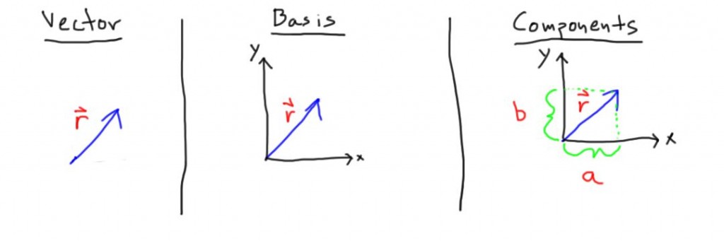
We can start with the abstract notion of a vector. We can think about a vectors as just an arrow that points in some direction with some length. This is a nice geometrical picture of a vectors, but it is difficult to use a picture to do a calculation. We want to turn our geometrical picture into the usual algebraic picture of vectors.
\(\vec r=a\hat x+b\hat y\)
Choosing a Basis
We will need to develop some tools to do this. One tool we will need is a basis. In our algebraic picture, choosing a basis means that we choose to describe our vector, \(\vec r\), in terms of the components in the \(\hat x\) and \(\hat y\) direction. As usual, we need our basis vectors to be linearly independent, have unit length, and we need one basis vector per dimension (they span the space).
Projection Operators
Now the question becomes: how can we calculate the components in the different directions? The way we learn to do this with vectors is by projection. So, we need projection operators. Things that eat our vector, \(\vec r\), and spit out the components in the \(\hat x\) and \(\hat y\) directions. For the example vector above, this would be:
We want these projection operators to have a few properties, and as long as they have these properties, any operator we can cook up will work. We want the projection operator in the \(x\) direction to only pick out the \(x\) component of our vector. If there is an \(x\) component, the projection operator should return it, and if there is no \(x\) component, it should return zero.
Great! Because we have used vectors before, we know that the projection operators are dot products with the unit vectors.
We can also check that these projection operators satisfy the properties that we wanted our operators to have.
So, now we have a way to take some arbitrary vector—maybe it was given to us in magnitude and angle form—and break it into components for our chosen basis.
Vector Rebuilder
The last tool we want is a way of taking our components and rebuilding our vector in our chosen basis. I don’t know of a mathematical name for this, so I’m going to call it a vector rebuilder. We know how to do this with our basis unit vectors:
\(\vec r = a\hat x+b\hat y = \text{Proj}_x(\vec r) \hat x+\text{Proj}_y(\vec r)\hat y = \sum_{e=x,y}\text{Proj}_e(\vec r)\hat e.\)
So, to recap, we have developed three tools:
Basis: chosen set of unit vectors that allow us to describe any vector as a unique linear combination of them.
Projection Operators: set of operators that allow us to calculate the components of a vector along any basis vector.
Vector Rebuilder: expression that gives us our vector in terms of our basis and projection operators.
This may seem silly or overly pedantic, but during Part 2, I’ll (hopefully) make it clear how we can develop these same tools for Fourier analysis and use them to gain some intuition for the goals and techniques used.