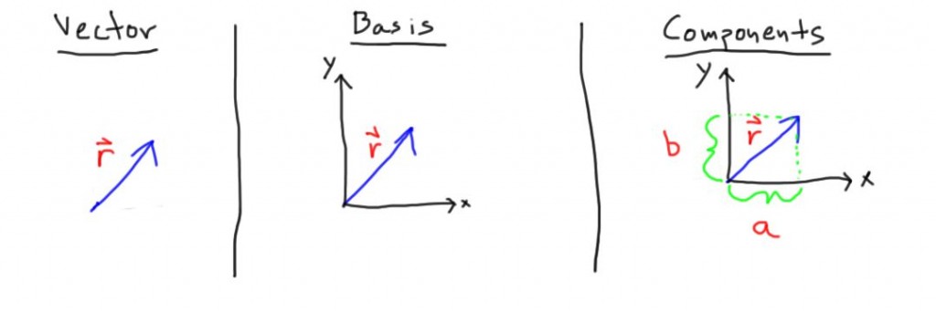
In Part 2, we adapted three tools developed for vectors to functions: a Basis in which to represent our function, Projection Operators to find the components of our function, and a Function Rebuilder which allows us to recreate our vector in the new basis. This is the third (and final!) post in a series of three:
- Part 1: Developing tools from vectors
- Part 2: Using these tools for Fourier series
- Part 3: A few examples using these tools
We can apply these tools to two problems that are common in Fourier Series analysis. First we’ll look at the square wave and then the sawtooth wave. Since we’ve chosen a sine and cosine basis (a frequency basis), there are a few questions we can ask ourselves before we begin:
- Will these two functions contain a finite or infinite number of components?
- Will the amplitude of the components grow or shrink as a function of their frequency?
Let’s try and get an intuitive answer to these questions first.
For 1., another way of asking this question is “could you come up with a way to combine a few sines and cosines to create the function?” The smoking guns here are the corners. Sines and cosines do not have sharp corners and so making a square wave or sawtooth wave with a finite number of them should be impossible.
For 2., one way of thinking about this is that the function we are decomposing are mostly smooth with a few corners. To get them to be smooth, we can’t have more and more high frequency components, so the amplitude of the components should shrink.
Let’s see if these intuitive answers are borne out.
Square Wave
We’ll center the square wave vertically at zero and let it range from \([-L, L]\). In this case, the square wave function is
\(f(x)=\begin{cases}1&-L\leq x\leq 0 \\-1&0\leq x\lt L\end{cases}.\)
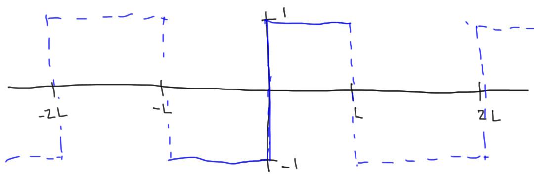
If we imagine this function being repeated periodically outside the range \([-L, L]\), it would be an odd (antisymmetric) function. Since sine functions are odd and cosine functions are even, an arbitrary odd function should only be built out of sums of other odd functions. So, we get to take one shortcut and only look at the projections onto the sine function (the cosine projections will be zero). You should work this out if this explanation wasn’t clear.
Since the square wave is defined piecewise, our projection integral will also be piecewise:
\(a_n = \text{Proj}_{s_n}(f(x)) \\= \int_{-L}^{0}dx\frac{1}{\sqrt{L}} \sin(\frac{n\pi x}{L}) (1)+\int_{0}^Ldx\frac{1}{\sqrt{L}} \sin(\frac{n\pi x}{L})(-1).\)
Both of these integrals can be done exactly.
\(a_n = \frac{1}{\sqrt{L}} \frac{-L}{n \pi}\cos(\frac{n\pi x}{L})|_{-L}^0 +\frac{1}{\sqrt{L}} \frac{L}{n \pi}\cos(\frac{n\pi x}{L})|_0^L \\= -\frac{\sqrt{L}}{n \pi}\cos(0)+\frac{\sqrt{L}}{n \pi}\cos(-n\pi)+\frac{\sqrt{L}}{n \pi}\cos(n\pi)-\frac{\sqrt{L}}{n \pi}\cos(0)\\= \frac{2\sqrt{L}}{n \pi}\cos(n\pi)-\frac{2\sqrt{L}}{n \pi}\cos(0).\)
\(\cos(n\pi)\) will be \((-1)^{n}\) and \(\cos(0)\) is \(1\). And so we have
\(a_n=\frac{4\sqrt{L}}{n \pi}\begin{cases}1&n~\text{odd}\\ 0 &n~\text{even}\end{cases}.\)
\(f(x)=\sum_{1,3, 5,\ldots}\frac{4}{n \pi}\sin(\frac{n\pi x}{L})\)
So we can see the answer to our questions. The square wave has an infinite number of components and those components shrink as \(1/n\).
Sawtooth Wave
We’ll have the sawtooth wave range from -1 to 1 vertically and span \([-L, L]\). In this case, the sawtooth wave function is
\(g(x)=\frac{x}{L}.\)

This function is also odd. The sawtooth wave coefficients will only have one contributing integral:
\(a_n = \text{Proj}_{s_n}(f(x)) = \int_{-L}^Ldx\sqrt{\frac{1}{L}} \sin(\frac{n\pi x}{L})\frac{x}{L}.\)
This integral can be done exactly with integration by parts.
\(a_n = \sqrt{\frac{1}{L}}(-\frac{x}{n \pi}\cos(\frac{n\pi x}{L})+\frac{L}{n^2 \pi^2}\sin(\frac{n\pi x}{L}))|_{-L}^L\\=(-\frac{\sqrt{L}}{n \pi}\cos(n\pi)+\frac{\sqrt{L}}{n^2 \pi^2}\sin(n\pi))-(\frac{\sqrt{L}}{n \pi}\cos(n\pi)-\frac{\sqrt{L}}{n^2 \pi^2}\sin(n\pi))\\=\frac{2\sqrt{L}}{n^2 \pi^2}\sin(n\pi)-\frac{2\sqrt{L}}{n \pi}\cos(n\pi)\).
\(\cos(n\pi)\) will be \((-1)^n\) and \(\sin(n\pi)\) will be 0. And so we have
\(a_n=(-1)^{n+1}\frac{2\sqrt{L}}{n \pi}\)
\(g(x)=\sum_n(-1)^{n+1}\frac{2}{n \pi}\sin(\frac{n\pi x}{L})\)
Again we see that an infinite number of frequencies are represented in the signal but that their amplitude falls off at higher frequency.