Category: Machine Learning

Machine learning is a broad set of techniques which can be used to identify patterns in data and use these patterns to help with some task like early seizure-detection/prediction, automated image captioning, automatic translation, etc. Most machine learning techniques have a set of parameters which need to be tuned. Many of these techniques rely on a very simple idea from calculus in order to tune these parameters.

Machine learning is a mapping problem

Machine learning algorithms generally have a set of parameters, which we’ll call $$\theta$$, that need to be tuned in order for the algorithm to perform well at a particular task. An important question in machine learning is how to choose the parameters, $$\theta$$, so that my algorithm performs the task well. Let’s look at a broad class of machine learning algorithms which take in some data, $$X$$, and use that data to make a prediction, $$\hat y$$. The algorithm can be represented by a function which makes these predictions,

\( \hat y = f(X;\theta)\).

This notation means that we have some function or mapping $$f(.; \theta)$$ which has parameters $$\theta$$. Given some piece of data $$X$$, the algorithm will made some prediction $$\hat y$$. If we change the parameters, $$\theta$$, then the function will produce a different prediction.

If we choose random values for $$\theta$$, there is no reason to believe that our mapping, $$f(.; \theta)$$, will do anything useful. But, in machine learning, we always have some training data which we can use to tune the parameters, $$\theta$$. This training data will have a bunch of input data which we can label as: $$X_i,\ i \in 1,\ 2,\ 3,\ldots$$, and a bunch of paired labels: $$y_i,\ i \in 1,\ 2,\ 3,\ldots$$, where $$y_i$$ is the correct prediction for $$X_i$$. Often, this training data has either been created by a simulation or labeled by hand (which is generally very time/money consuming).

Learning is parameter tuning

Now that we have ground-truth labels, $$y_i$$, for our training data, $$X_i$$, we can then evaluate how bad our mapping, $$f(.; \theta)$$, is. There are many possible ways to measure how bad $$f(.; \theta)$$ is, but a simple one is to compare the prediction of the mapping $$\hat y_i$$ to the ground-truth label $$y_i$$,

\( y_i-\hat y_i \).

Generally, mistakes which cause this error to be positive or negative are equally bad so a good measure of the error would be:

\(( y_i-\hat y_i)^2 =( y_i-f(X_i;\theta))^2\).

When this quantity is equal to zero for every piece of data we are doing a perfect mapping, and the larger this quantity is the worse our function is at prediction. Let’s call this quantity summed over all of the training data the error

\(E(\theta)=\sum_i( y_i-f(X_i;\theta))^2\).

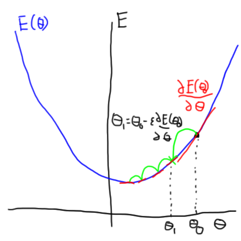
So, how do we make this quantity small? One simple idea from calculus is called gradient descent. If we can calculate the derivative or gradient of the error with respect to $$\theta$$ then we know that if we go in the opposite direction (downhill), then our error should be smaller. In order to calculate this derivative, our mapping, $$f(.,\theta)$$, needs to be differentiable with respect to $$\theta$$.

So, if we have a differentiable $$f(.,\theta)$$ we can compute the gradient of the cost function with respect to $$\theta$$

\(\frac{\partial E(\theta)}{\partial \theta}=\frac{\partial}{\partial \theta}\sum_i( y_i-f(X_i;\theta))^2=-2\sum_i( y_i-f(X_i;\theta))\frac{\partial f(X_i;\theta)}{\partial \theta}\).

If we have this derivative, we can then adjust our parameters, $$\theta^t$$ such that our error is a bit smaller

\(\theta^{t+1} = \theta^t – \epsilon\frac{\partial f(X_i;\theta)}{\partial \theta}\)

where $$\epsilon$$ is a small scalar. Now, if we repeat this process over and over, the value of the error, $$E(\theta)$$ should get smaller and smaller as we keep updating $$\theta$$. Eventually, we should get to a (local) minimum at which point our gradients will become zero and we can stop updating the parameters. This process is shown (in a somewhat cartoon way) in this figure.

Extensions and exceptions

This post presented a slightly simplified picture of learning in machine learning. I’ll briefly mention a few of the simplifications.

The terms error function, objective function, and cost function are all used basically interchangeably in machine learning. In probabilistic models you may also see likelihoods or log-likelihoods which are similar to a cost function except they are setup to be maximized rather than minimized. Since people (physicists?) like to minimize things, negative log-likelihoods are also used.

The squared-error function was a somewhat arbitrary choice of error function. It turns out that depending on what sort of problem you are working on, e.g. classification or regression, you may want a different type of cost function. Many of the commonly used error function can be derived from the idea of maximum likelihood learning in statistics.

There are many extensions to simple gradient descent which are more commonly used such as stochastic gradient descent (sgd), sgd with momentum and other fancier things like Adam, second-order methods, and many more methods.

Not all learning techniques for all models are (or were initially) done through gradient descent. The first learning rule for Hopfield networks was not based on gradient descent although the proof of the convergence of inference was based on (not-gradient) descent. Infact, it has been replaced with a more modern version based on gradient descent of an objective function.